TD1 - Bilan de liaison

1 - Introduction

Limiting link	-	UL
UL ratio	$p_{UL}$	0.2
Target cell edge data rate [Mbps]	$D$	20.0
Carrier frequency [GHz]	$f_c$	28
Allocated bandwidth [MHz]	$W$	100
BS antenna height [m]	$h_b$	33
UE antenna height [m]	$h_m$	1.50
Coverage probability	$p_c$	0.90
NLOS propagation	-	YES
Indoor coverage	-	NO
Shadowing standard deviation [dB]	$\sigma$	6
Number of HARQ retransmissions	$N_h$	4

2 - Transmission

1. Compute the EIRP and the transmit diversity gain

On a $P_{tx} = 23 dBm$ et $N_a = 2$

$$EIRP = P_{tx} + G_{tx} - L\\$$

Transmit diversity gain :

$$G_{tx} = 10 \log_{10} (N_{tx})\\$$

On calcule :

$$\begin{align*} & EIRP = 23 + 10 \log_{2} - 0\\ & EIRP = 23 + 3.01\\ & EIRP = 26.01 dBm\\ \end{align*}$$

3 - Reception

2. Compute the target SINR.

$$SNR = 10 \log_{10}(\beta (2^{\frac{C_{cible}}{\alpha W}}- 1 ))$$

On utilise $p_{UL}$ et $D$ de l'énoncé

$$C_{cible} = \frac{D}{p_{UL}} = \frac{20}{0.2} = 100 Mbps$$

On connait $\alpha = 1$ et $\beta = 1$ et $W = 100 MHz$

$$\begin{align*} & SNR = 10 \log_{10}(1 (2^\frac{100}{1 \cdot 100}- 1 ))\\ & SNR = 10 \log_{10}(2^\frac{100}{100}- 1 )\\ & SNR = 10 \log_{10}(2^1- 1 )\\ & SNR = 10 \log_{10}(2- 1 )\\ & SNR = 10 \log_{10}(1)\\ & SNR = 10 \cdot 0\\ & SNR = 0\\ \end{align*}$$

D'après l'énoncé, on a $L_i = 3 dB$

$$\begin{align*} & SINR_{cible} = SNR + L_{i}\\ & SINR_{cible} = 0 + 3\\ & SINR_{cible} = 3 dB\\ \end{align*}$$

3. Compute the noise power at the receiver.

On a

• $N_0 = -174 dBm/Hz$
• $W = 100 MHz$
• $N_F = 3 dB$

En $W$

$$\begin{align*} & N = N_0 \cdot W \cdot N_F\\ \end{align*}$$

En $dBm$ :

$$\begin{align*} & N = -174 + 10 \cdot \log(W) + N_F\\ & N = -174 + 10 \cdot \log(100 \cdot 10^6) + 3\\ & N = -174 + 10 \cdot 8 + 3\\ & N = -174 + 80 + 3\\ & N = -91 dBm\\ \end{align*}$$

4. Compute the receive array gain, the receive antenna gain and the diversity gain.

On a

• $Nb_{AE} = 128$
• $Nb_{AP} = 2$
• $G_{ae} = 8 dBi$

$$\begin{align*} & G_{array} = 10 \cdot \log_{10}(\frac{Nb_{AE}}{Nb_{AP}})\\ & G_{array} = 10 \cdot \log_{10}(\frac{128}{2})\\ & G_{array} = 10 \cdot \log_{10}(\frac{128}{2})\\ & G_{array} = 10 \cdot 1.80617997398\\ & G_{array} = 18.06 dB\\ \end{align*}$$ $$\begin{align*} & G_{diversity} = 10 \cdot \log_{10}(Nb_{AP})\\ & G_{diversity} = 10 \cdot \log_{10}(2)\\ & G_{diversity} = 10 \cdot 0.301\\ & G_{diversity} = 3.01 dB\\ \end{align*}$$

Le gain de l'antenne de réception correspond au gain d'un élément d'antenne $G_{ae} = 8 dBi$

5. After including typical scheduling gain and HARQ gain, compute the sensitivity of the receiver.

La valeur typique du gain d'ordonnancement est de $G_s = 3dB$

Dans l'énoncé on a $N_h = 4$

$$\begin{align*} & G_{HARQ} = 10 \cdot \log_{10}(N_h)\\ & G_{HARQ} = 10 \cdot \log_{10}(4)\\ & G_{HARQ} = 6 dB\\ \end{align*}$$ $$\begin{align*} & S = SINR + N - G\\ & S = SINR + N - G_{array} - G_{diversity} - G_{ae} - G_s - G_{HARQ}\\ & S = 3 +(-91) - 18.06 - 3.01 - 8 - 3 - 6\\ & S = -126.07 dBm\\ \end{align*}$$

4 - Margins

6. Compute the shadowing margin.

On connait

• d'après l'énoncé $\sigma = 6 dB$
• d'après l'énoncé $p_c = 0.9$
• $P_{out} = 1 - p_c = 1 - 0.9 = 0.1$

On utilise la formule de Jakes

$$\begin{align*} & K_s = \sigma Q^{-1}(P_{out}) \end{align*}$$

On sait que $Q^{-1}(0.1) = 1.28$

$$\begin{align*} & K_s = 6 Q^{-1}(0.1) & K_s = 6 \cdot 1.28 & K_s = 7.68 dB \end{align*}$$

7. Refer to Raghavan et al., 2019 and propose a hand and body loss for our link budget.

On utilise les valeurs de la table 1 de l'article

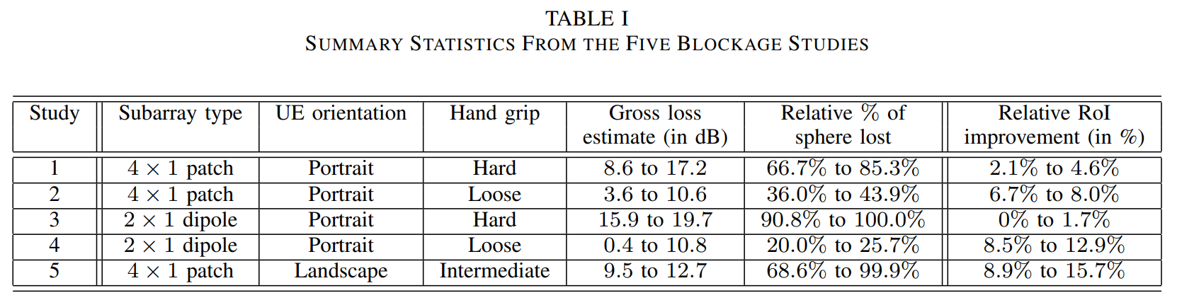
On regarde les lignes Subarray type 2 x 1 dipole. On choisit de prendre le “Hard Hand Grip” car c'est le pire des cas

On a donc $K_{hl}=15dB$

8. Compute the indoor penetration loss when indoor coverage is required up to 1m.

On regarde le modele 3GPP 38901-g10-channel-models.pdf et on utilise le O2I building penetration loss.

On a $f_c = 28$

$$PL = PL_b + PL_{tw} + PL_{in} + N(0, \sigma^2_P)$$ $$PL_{in} = 0.5 \cdot d = 0.5 dB$$

On utilise le modèle de low-loose model pour $PL_{tw}$ (d'après l'article):

$$\begin{align*} & PL_{tw} = 5 - 10\log_{10} (p_{glass} \cdot 10^{\frac{-L_{\mathrm{glass}}}{10}} + p_{concrete} \cdot 10^{\frac{-L_{\mathrm{concrete}}}{10}}) \\ & PL_{tw} = 5 - 10\log_{10} (0.3 \cdot 10^{\frac{-(2+0.2*f_c)}{10}} + 0.7 \cdot 10^{\frac{-(5+4*f_c)}{10}}) \\ & PL_{tw} = 5 - 10\log_{10} (0.3 \cdot 10^{\frac{-(2+0.2*28)}{10}} + 0.7 \cdot 10^{\frac{-(5+4*28)}{10}}) \\ & PL_{tw} = 5 - 10\log_{10} (0.3 \cdot 10^{\frac{3.6}{10}} + 0.7 \cdot 10^{\frac{5+4*28}{10}}) \\ & PL_{tw} = 5 - 10\log_{10} (0.3 \cdot 10^{0.36} + 0.7 \cdot 10^{\frac{117}{10}}) \\ & PL_{tw} = 5 - 10\log_{10} (0.3 \cdot 10^{0.36} + 0.7 \cdot 10^{11.7}) \\ & PL_{tw} = 17.8 dB \\ \end{align*}$$

On trouve donc $PL = 0.5 + 17.8 = 18.3 dB$

9. Refer to Bas et al., 2018 and propose a foliage loss for our link budget.

On a $d_v$ = 2m$

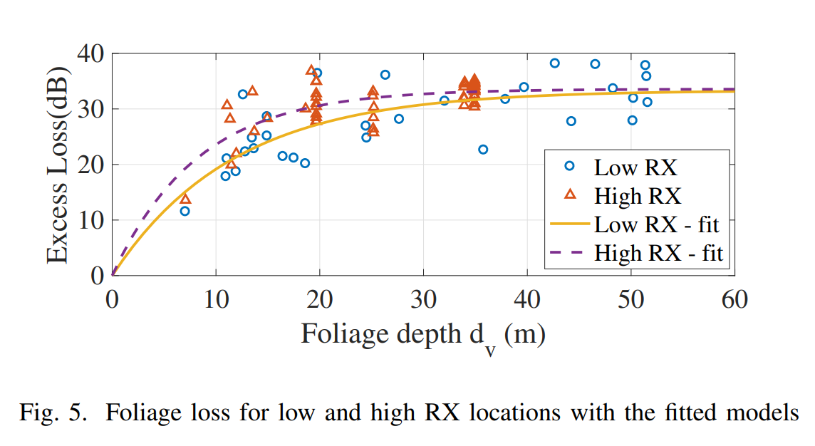
On trouve donc $4.5 dB$

10. Refer to Azar et al., 2013 and propose a rain loss for our link budget.

On connait $f_c = 28 GHz$

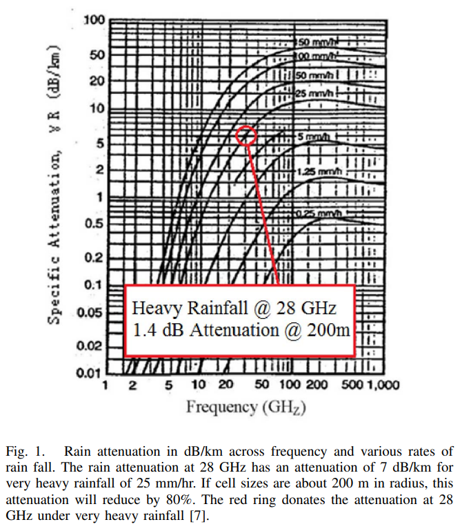
On trouve donc $Rain_{loss} = 1.4 dB$

5 - Cell radius

11. Compute the MAPL and the cell range indoor and outdoor.

Modele 3GPP 38901-g10-channel-models.pdf.

On connait

• $PIRE = 26.01 dBm$
• $S = -126.07 dBm$
• $M_i = 0.5 dB$
• $K_s = 7.68 dB$ - shadowing margin
• $G_{array} = 18.06 dB$
• $G_{diversity} = 3.01 dB$
• $G_{ae} = 8 dBi$
• $K_{hl} = 15dB$ - hand and body loss
• $F_{loss} = 4.5 dB$
• $Rain_{loss} = 1.4 dB$
• $PL = 18.3 dB$ - indoor penetration loss

Cas "cell range indoor" :

$$\begin{align*} & MAPL = PIRE - S - Marges - Pertes + Gain\\ & MAPL = 26.01 - (-126.07) - M_i - K_s - K_{hl} - PL - F_{loss} - Rain_{loss} + \\ & MAPL = 26.01 - (-126.07) - 0.5 - 7.68 - 15 -18.3 - 4.5 - 1.4\\ & MAPL = 104.7 dB\\ \end{align*}$$

Cas "cell range outdoor" :

$$\begin{align*} & MAPL = PIRE - S - Marges - Gains - Pertes\\ & MAPL = 26.01 - (-126.07) - M_i - K_s - K_{hl} - F_{loss} - Rain_{loss}\\ & MAPL = 26.01 - (-126.07) - 0.5 - 7.68 - 15 - 4.5 - 1.4\\ & MAPL = 123 dB\\ \end{align*}$$

On utilise la formule de NLOS propagation :

$$PL_{UMA-NLOS} = 13.54 + 39.08 \log_{10}(d_{3D}) + 20 \log_{10}(f_c) - 0.6(h_{UT} - 1.5)$$

On inverse la formule pour avoir donc :

$$d_{3D} = 10^{\frac{PL_{UMA-NLOS} - 13.54 - 20 \log_{10}(28) + 0.6(h_{UT} - 1.5)}{39.08}}$$

On connait aussi :

• $h_{BS} = 33 m$
• $h_{UT} = 1.5 m$
• $f_c = 28 GHz$

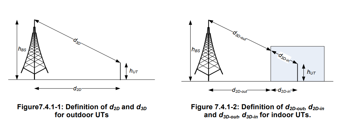
Or nous voulons pour $d_{2D}$

$$d_{2D} = \sqrt{(d_{3D})^{2} - (h_{BS} - h_{UT})^{2}}$$

On trouve donc $d_{3D-in} = 39.09m$ et $d_{2D-in} = 23.14m$

On trouve donc $d_{3D-out} = 114.9m$ et $d_{2D-out} = 110.5m$

6 - Deployment scenario in Paris 13

12. Deployment scenario in Paris 13

On connait :

• la formule de l'aire d'un cercle : $S = \pi \cdot R^2$ donc la formule du rayon d'un cercle : $\sqrt{\frac{S}{\pi}}$
• la surface de Paris 13 : $7.15 km^2$
• le nombre de sites LTE : 31

Surface moyenne d'une cellule :

$$\begin{align*} & S_{moy} = \frac{Aire_{Paris13}}{Nb_{LTE}}\\ & S_{moy} = \frac{7.15}{31}\\ & S_{moy} = 0.230 km^2\\ \end{align*}$$

Le rayon moyen d'une cellule :

$$\begin{align*} & R_{moy} = \sqrt{\frac{S_{moy}}{\pi}}\\ & R_{moy} = \sqrt{\frac{0.230}{\pi}}\\ & R_{moy} = \sqrt{0.073}\\ & R_{moy} = 0.27 km\\ & R_{moy} = 270 m\\ \end{align*}$$

13. What is the proportion of Paris 13 area that could be covered with mmW if only LTE sites were reused?

$$\begin{align*} & Aire_{moy} = Nb_{LTE} \cdot \pi \cdot d_{2D-out}^{2}\\ & Aire_{moy} = 31 \cdot \pi \cdot (110.5*10^{-3})^{2}\\ & Aire_{moy} = 1.18 km^2\\ \end{align*}$$ $$\begin{align*} & Proportion = \frac{Aire_{moy}}{Aire_{Paris13}}\\ & Proportion = \frac{0.46}{7.15}\\ & Proportion = 16\%\\ \end{align*}$$

14. How many mmW sites would be needed to cover the whole area?

$$\begin{align*} & Nb_{site} = \frac{Aire_{Paris13}}{Aire_{cell}}\\ & Nb_{site} = \frac{Aire_{Paris13}}{\pi \cdot d_{2D-out}^{2}}\\ & Nb_{site} = \frac{7.15}{\pi \cdot (110.5*10^{-3})^{2}}\\ & Nb_{site} = 186\\ \end{align*}$$

15. Same questions if the target cell edge data rate is set to 5 Mbps.

$$\begin{align*} & C_{cible} = \frac{5}{0.2} = 25 Mbps\\ & SNR = 10 \log_{10}(2^\frac{25}{1 \cdot 100}- 1 ) = -7.23 dB\\ & SINR = -7.23 + 3 = -4.23 dB\\ & S = -133.3 dBm\\ & MAPL_{out} = 130.23 dB\\ & d_{3D-out} = 173.6m\\ & d_{2D-out} = 170.7m\\ & Nb_{site} = 7.15 / (\pi \cdot (170.7*10^{-3})^{2}) = 78\\ \end{align*}$$

16. Same questions if the target cell edge data rate is set to 5 Mbps and indoor coverage is required.

$$\begin{align*} & C_{cible} = \frac{5}{0.2} = 25 Mbps\\ & SNR = 10 \log_{10}(2^\frac{25}{1 \cdot 100}- 1 ) = -7.23 dB\\ & SINR = -7.23 + 3 = -4.23 dB\\ & S = -133.3 dBm\\ & MAPL_{indoor} = 111.93 dB\\ & d_{3D-out} = 59.85m\\ & d_{2D-out} = 50.9m\\ & Nb_{site} = 7.15 / (\pi \cdot (170.7*10^{-3})^{2}) = 878\\ \end{align*}$$